EXPLAIN prints the planner’s proposed execution plan; EXPLAIN ANALYZE executes the statement and adds measured rows and times. A slow query needs both a hypothesis and a measurement. Save the query parameters, PostgreSQL version, and original plan before changing an index or rewriting a join. Those details make the next plan comparable and prevent an improvement on one input from hiding a regression on another.
Compare estimated and actual rows, but treat a gap as evidence to interpret, not the diagnosis itself. Loops and early stopping can explain apparently different counts. Accurate estimates also coexist with expensive work, lock waits, or spills. Change one variable at a time and preserve the before-and-after results so the proposed explanation can be tested.

Read the shape top-down or leaves-first
Text output prints a parent before its indented children. Read downwards to understand which inputs a node consumes, then follow rows upwards to understand the result. Execution can be demand-driven: a LIMIT may stop requesting rows early, while a sort often needs its entire input before returning anything. Indentation describes dependencies, not a universal chronological execution order.
Costs use planner units, not milliseconds. A node’s total cost includes its children, so adding every displayed cost double-counts work. Startup cost estimates the work before the first row; total cost estimates completing the node. Actual times and rows are averages per execution when loops exceeds one. Multiply by loops when judging repeated work, and remember that parent timing also includes descendant work.
Recognize scans, joins, sorts, aggregates, and limits, then inspect their inputs. A nested loop with a selective inner index can be appropriate; a hash join can spill to multiple batches. The node name does not establish whether its work is excessive for this result.
Follow the work and amplification
The largest row count is a clue, not proof of the bottleneck. A cheap sequential scan can outperform many random index reads; a small node repeated thousands of times can dominate a query. Find the first substantial estimated-versus-actual row mismatch, then trace its effect on joins, sorting, and memory use. Check buffers and temporary reads or writes before deciding whether storage access, repeated execution, or a spill explains the delay.
The planner chooses among explored alternatives using a cost model; statistics are one input. Inspect pg_stats for skew or stale estimates, and consider correlations between columns. Extended statistics can describe some same-table relationships, but do not fix every estimate or generally supply cross-table join selectivity. Verify that the proposed statistics actually change the relevant estimate before crediting them.
Bind rows to cost with ANALYZE
EXPLAIN ANALYZE runs the real query. Large row-estimation errors can come from stale statistics, skew, or correlations between columns. Refreshing statistics may help, but does not guarantee a fix. Extended statistics can describe some correlations; a representative test must still confirm the chosen plan and result. An index is justified by the access pattern and measured cost, not just by seeing many filtered rows.
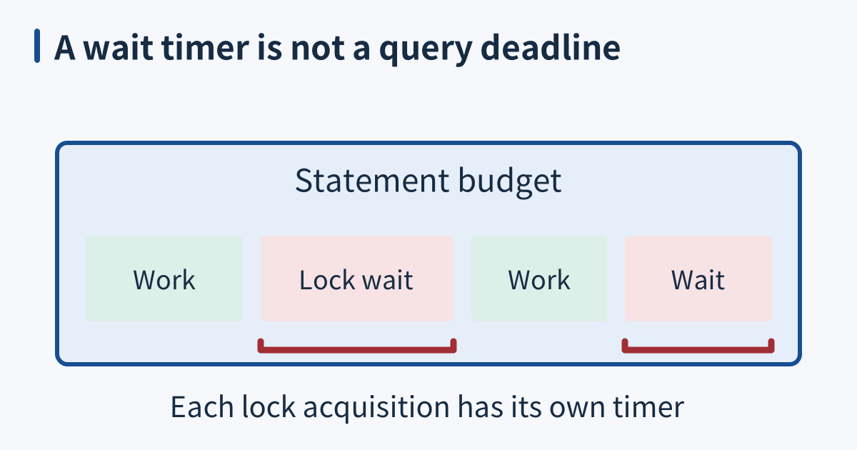
Use an isolated database for write experiments. Rolling back table changes does not undo sequence allocation or external effects from functions and triggers. Even a SELECT can call a function with side effects. Set a statement timeout, understand the statement, and use plain EXPLAIN first when execution cost is uncertain. Buffer reads also do not prove physical disk I/O: the operating system may satisfy them from its cache.
When it breaks
Tuning the wrong statement wastes effort. Rank workload costs, for example with pg_stat_statements, then connect candidates to actual slow requests. A statement with high cumulative time may simply run frequently; that ranking alone does not explain a particular request’s tail latency. Include call counts, representative parameters, and request tracing when choosing the target.
Another failure is parameter sensitivity: one tenant is tiny and another holds most rows, while a prepared statement’s generic plan treats both alike. Compare representative parameters through the same prepared-statement path used by the application. PostgreSQL core has no general SQL hint syntax; investigate statistics, query shape, and generic versus custom plans before changing planner settings globally.
Check it quickly
In a writable scratch database, create data owned only by this session:
BEGIN;
SET LOCAL statement_timeout = '10s';
CREATE TEMP TABLE explain_demo AS
SELECT n AS id, n % 100 AS tenant_id FROM generate_series(1, 20000) AS g(n);
ANALYZE explain_demo;
EXPLAIN (ANALYZE, BUFFERS)
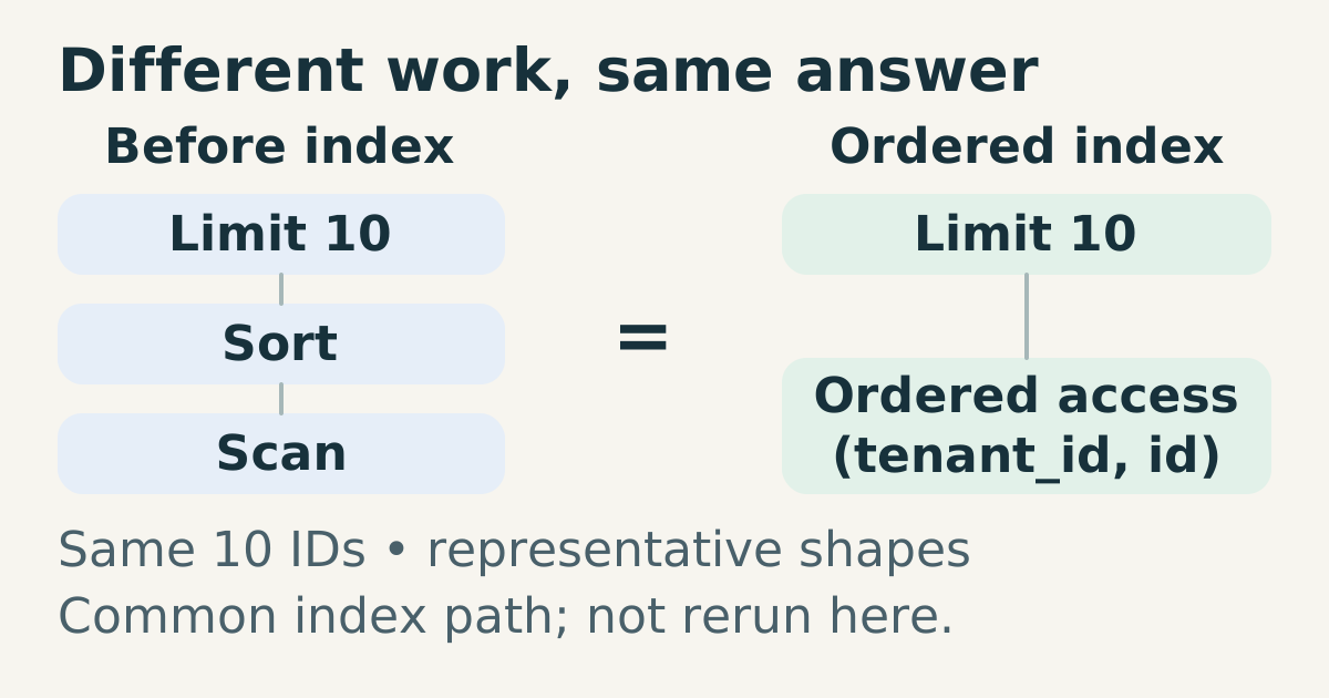
SELECT id FROM explain_demo WHERE tenant_id = 17 ORDER BY id LIMIT 10;
SELECT id FROM explain_demo WHERE tenant_id = 17 ORDER BY id LIMIT 10;
CREATE INDEX explain_demo_lookup ON explain_demo (tenant_id, id);
EXPLAIN (ANALYZE, BUFFERS)
SELECT id FROM explain_demo WHERE tenant_id = 17 ORDER BY id LIMIT 10;
SELECT id FROM explain_demo WHERE tenant_id = 17 ORDER BY id LIMIT 10;
ROLLBACK;
Both queries must return IDs 17 through 917 at intervals of 100, in that order. Compare scan type, sort presence, rows filtered, and buffers; the second plan will commonly use the ordered index. Do not require an exact time or node shape across versions. Repeat on representative data before applying the index to a real workload; rollback removes this experiment.
Sources
PostgreSQL EXPLAIN documentation, EXPLAIN options and execution side effects, checked 2026-10-15.
PostgreSQL using EXPLAIN, plan trees, row estimates, loops and measured costs, checked 2026-10-15.
PostgreSQL 18: Extended statistics, same-table correlations and ANALYZE collection, checked 2026-10-15.
PostgreSQL 18: CREATE STATISTICS, statistics kinds and the table-join selectivity limitation, checked 2026-10-15.
PostgreSQL 18: pg_stat_statements, call counts and cumulative execution time, checked 2026-10-15.